ملف:Partial transmittance.gif
لا توجد دقة أعلى متوفرة.
Partial_transmittance.gif (367 × 161 بكسل حجم الملف: 67 كيلوبايت، نوع MIME: image/gif، ملفوف، 53 إطارا، 4٫2ث)
| هذا ملف من ويكيميديا كومنز. معلومات من صفحة وصفه مبينة في الأسفل. كومنز مستودع ملفات ميديا ذو رخصة حرة. |
ملخص
| الوصف |
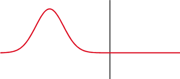
Русский: Показано классическое отражение/прохождение солитона гауссового импульса от/в более плотную среду. В реальности же, свет отражается не от поверхности, а от всех частиц тела (см. ru:КЭД). English: Illustration of partial reflection of a wave. A gaussian wave on a one-dimensional string strikes a boundary with transmission coefficient of 0.5. Half the wave is transmitted and half is reflected.
Français : Illustration de la réflection partielle d'une onde. Une onde gaussienne se déplaçant sur un ressort unidimensionnel est réfléchie/transmise au niveau d'une interface avec un coefficient de transmission de 0.5.
Español: Ilustración de una reflexión parcial de una onda. Una onda gaussiana sobre una cuerda de una dimensión choca contra un limite con un coeficiente de transmisión de 0.5. La mitad de la onda es transmitida y la otra mitad es reflejada. |
| التاريخ | |
| المصدر | self-made with MATLAB, source code below |
| المؤلف | Oleg Alexandrov |
.هذا الرسم المتجهي أُنشئ بواسطة MATLAB
ترخيص
| أنا، مالِك حقوق تأليف ونشر هذا العمل، أجعله في النِّطاق العامِّ، يسري هذا في أرجاء العالم كلِّه. في بعض البلدان، قد يكون هذا التَّرخيص غيرَ مُمكنٍ قانونيَّاً، في هذه الحالة: أمنح الجميع حق استخدام هذا العمل لأي غرض دون أي شرط ما لم يفرض القانون شروطًا إضافية. |
MATLAB source code
% Partial transmittance and reflectance of a wave
% Code is messed up, don't have time to clean it now
function main()

   % KSmrq's colors
   red    = [0.867 0.06 0.14];
   blue   = [0, 129, 205]/256;
   green  = [0, 200,  70]/256;
   yellow = [254, 194,   0]/256;
   white = 0.99*[1, 1, 1];
   black = [0, 0, 0];

   % length of the string and the grid
   L = 5;
   N = 151;
   X=linspace(0, L, N);

   h = X(2)-X(1); % space grid size
   c = 0.01; % speed of the wave
   tau = 0.25*h/c; % time grid size

   % form a medium with a discontinuous wave speed
   C = 0*X+c;

   D=L/2;
   c_right = 0.5*c; % speed to the right of the disc
   for i=1:N
      if X(i) > D
         C(i) = c_right;
      end
   end
   % Now C = c for x < D, and C=c_right for x > D

   K = 5; % steepness of the bump
   S = 0; % shift the wave
   f=inline('exp(-K*(x-S).^2)', 'x', 'S', 'K'); % a gaussian as an initial wave
   df=inline('-2*K*(x-S).*exp(-K*(x-S).^2)', 'x', 'S', 'K'); % derivative of f

   % wave at time 0 and tau
   U0 = 0*f(X, S, K);
   U1 = U0 - 2*tau*c*df(X, S, K);

   U = 0*U0; % current U

   % plot between Start and End
   Start=130; End=500;

   % hack to capture the first period of the wave
   min_k = 2*N; k_old = min_k; turn_on = 0;

   frame_no = 0;
   for j=1:End

      %  fixed end points
      U(1)=0; U(N)=0;

      % finite difference discretization in time
      for i=2:(N-1)
         U(i) = (C(i)*tau/h)^2*(U1(i+1)-2*U1(i)+U1(i-1)) + 2*U1(i) - U0(i);
      end

      % update info, for the next iteration
      U0 = U1; U1 = U;

      spacing=7;

     % plot the wave
      if rem(j, spacing) == 1 & j > Start

         figure(1); clf; hold on;
         axis equal; axis off;
         lw = 3; % linewidth

         % size of the window
         ys = 1.2;

         low = -0.5*ys;
         high = ys;
         plot([D, D], [low, high], 'color', black, 'linewidth', 0.7*lw)
%         fill([X(1), D, D, X(1)], [low, low, high, high], [0.9, 1, 1], 'edgealpha', 0);
%         fill([D X(N), X(N), D],  [low, low, high, high], [1, 1, 1], 'edgealpha', 0);

         plot(X, U, 'color', red, 'linewidth', lw);

         % plot the ends of the string
         small_rad = 0.06;

         axis([-small_rad, 0.82*L, -ys, ys]);

         % small markers to keep the bounding box fixed when saving to eps
         plot(-small_rad, ys, '*', 'color', white);
         plot(L+small_rad, -ys, '*', 'color', white);

         pause(0.1)
         frame_no = frame_no + 1;
         %frame=sprintf('Frame%d.eps', 1000+frame_no); saveas(gcf, frame, 'psc2');
         frame=sprintf('Frame%d.png', 1000+frame_no);% saveas(gcf, frame);
         disp(frame)
         print (frame, '-dpng', '-r300');

      end
   end


% The gif image was creating with the command
% convert -antialias -loop 10000  -delay 8 -compress LZW -scale 20% Frame10*png Partial_transmittance.gif
% and was later cropped in Gimp
تاريخ الملف
اضغط على زمن/تاريخ لرؤية الملف كما بدا في هذا الزمن.
| زمن/تاريخ | صورة مصغرة | الأبعاد | مستخدم | تعليق | |
|---|---|---|---|---|---|
| حالي | 16:36، 9 أبريل 2010 | | 367 × 161 (67 كيلوبايت) | Aiyizo | optimized animation |
| 05:56، 26 نوفمبر 2007 |  | 367 × 161 (86 كيلوبايت) | Oleg Alexandrov | {{Information |Description=Illustration of en:Transmission coefficient (optics) |Source=self-made with MATLAB, source code below |Date=~~~~~ |Author= Oleg Alexandrov |Permission=PD-self, see below |other_versions= }} {{PD-se |
استخدام الملف
ال3 صفحات التالية تستخدم هذا الملف:
الاستخدام العالمي للملف
الويكيات الأخرى التالية تستخدم هذا الملف:
- الاستخدام في bg.wikipedia.org
- الاستخدام في ca.wikipedia.org
- الاستخدام في de.wikipedia.org
- Reflexion (Physik)
- Fresnelsche Formeln
- Zeitbereichsreflektometrie
- Anpassungsdämpfung
- Benutzer Diskussion:Bleckneuhaus
- Wikipedia Diskussion:WikiProjekt SVG/Archiv/2012
- Wellenwiderstand
- Benutzer:Ariser/Stehwellenverhältnis Alternativentwurf
- Benutzer:Herbertweidner/Stehwellenverhältnis Alternativentwurf
- Benutzer:Physikaficionado/Fresnelsche Formeln-Röntgenstrahlung
- الاستخدام في de.wikibooks.org
- الاستخدام في en.wikipedia.org
- الاستخدام في en.wikibooks.org
- الاستخدام في en.wikiversity.org
- Quantum mechanics/Timeline
- How things work college course/Quantum mechanics timeline
- Quantum mechanics/Wave equations in quantum mechanics
- MATLAB essential/General information + arrays and matrices
- WikiJournal of Science/Submissions/Introduction to quantum mechanics
- WikiJournal of Science/Issues/0
- Talk:A card game for Bell's theorem and its loopholes/Conceptual
- Wright State University Lake Campus/2019-1/Broomstick
- Physics for beginners
- MyOpenMath/Physics images
- الاستخدام في es.wikipedia.org
- الاستخدام في et.wikipedia.org
- الاستخدام في fa.wikipedia.org
- الاستخدام في fa.wikibooks.org
- الاستخدام في fr.wikipedia.org
- الاستخدام في he.wikipedia.org
- الاستخدام في hy.wikipedia.org
- الاستخدام في it.wikipedia.org
- الاستخدام في ko.wikipedia.org
اعرض المزيد من الاستخدام العام لهذا الملف.